


Introduction
I’ve recently become very interested in molecular dynamics, or MD.
Why would you want to do MD at all? MD allow you to watch molecules dance in full atomic detail. While experimental techniques give you static molecular mugshots, MD lets you observe the dynamic behavior of molecules over time. And understanding molecular motion is key for everything in biology, everything in biology is vibrating molecules underneath the surface! Beyond just watching, you can use MD to predict molecular behavior. Want to know how tightly a drug will bind its target? Run an MD simulation and calculate the binding free energy. Trying to design a new enzyme? Simulate different designs to see which folds and functions best. Obviously, there are limitations — as we’ll get into — but the possibilities the field presents are fascinating.
Unfortunately, MD also happens to be incredibly hard to learn on your own. Unlike my other posts, where I can go from nearly zero knowledge to blog-post-capable in a week, MD has taken me the better part of a month and I’m still unsure of a lot of things. I’m much more used to the general fuzziness of ML; extremely overparameterized statistical models that can actively learn means that their exact theoretical underpinnings are, at best, interesting, but rarely useful outside of a few cases. So, hand-waving is practically fine! This isn’t the case in MD, all of it feels important to know and understand. You’re dealing with physics after all, and even if you hand-wave away certain aspects of the physics, your simplified model will be that much less capable of understanding certain phenomena.
In this post, I’ll try to equip you with enough knowledge to run basic simulations on your own, while also having enough theoretical backing to understand what’s actually going on under the surface. Obviously, we’ll be skipping a lot of things, but there should be enough here to vaguely understand some MD papers! To test this out, we’ll also go over two MD papers at the end of the post.
How does MD work in practice?
Consider a protein that we dreamed up. Completely unfolded, just a straight line of amino-acids linked together, Glycine-Lysine-Alanine, and so on. What happens if we drop this protein in a bucket of water and wait a few hundred nanoseconds? It’ll slowly turn from a straight line into a knotted mess of tangles and curves. Or, in other words, it will fold.
Most people will be familiar with the concept of a protein folding, the Alphafold2 news-cycle hammered that into most of us. But it's worth considering what it means for a protein to 'want' to fold at all. In many ways, a protein 'wants' to fold in the same way a dropped apple 'wants' to fall to the ground — physics simply pulls it in that direction. In the case of the apple, gravity is making the biggest call. In the case of the protein, the forces at play are more at the molecular level. Here are some:
Bond forces: Chemical attachments between neighboring atoms that can be stretched, twisted, or turned to different angles.
Electrostatic interactions: Attractions or repulsion between charged atoms.
Van der Waals forces: Weak electromagnetic attractions between all atoms in close proximity
Solvent interactions: Some parts of a protein may be hydrophobic/hydrophilic and will desire to hide its hydrophobic elements away from water + expose its hydrophilic elements to water.
There’s a few more of course, but these are the major ones. These forces will push and pull on every atom contained in the protein, ultimately forcing it to a certain configuration. As mentioned, this final configuration is the folded state of the protein, but we could interpret this final state in a more physics-grounded way: low thermodynamic free energy. It’s not worth pondering too much how to quantitatively assess this, but rest assured there are, we’ll discuss it a bit more later. Low thermodynamic free energy of a folded structure means it’s a stable structure (hard to move from), and high means its an unstable structure (easy to move from).
To note, the above pushing-pulling on our protein isn’t just the case for protein folding, it’s for all problems! Docking with small molecules, chemical reactions, everything moves towards the direction of low thermodynamic free energy.
Let’s return to our protein though, how do we figure out the final folded state of our protein with MD? There’s some nuance here in that some proteins will have multiple states with low thermodynamic free energy states, so the equilibrium state for a protein could be flip-flopping between multiple states. Let’s ignore that for now and assume there is a singular final state for this specific protein.
System Definition
First, we dunk the protein in a big cube of water.
Computationally that is. This isn’t an oversimplification, you literally ‘define’ a 5x5x5 (or however large) nanometer cube filled with H20 molecules around your protein, or the solvent. Why water? Most proteins exist in aqueous environments, so this is just an attempt to match the ‘natural’ environment of a protein. This is important because the environment often defines what final states a protein can reach — there are many possible end states of a protein, but not all of them are reachable in all environments. Lots of simulations also add in various salts and ions in the solution to bring the overall charge of the cube of water + protein to neutral, as that’s also (mostly) biologically realistic. To note, water isn’t the only possible solvent, one can really use anything, like ethanol, it just depends on whether the MD software package you’re using supports that.
Two last things. One, you may often hear the phrase ‘periodic boundary condition’ when it comes to the definition of this box of water, this just means that the box will loop any molecule that touches a side to the other side of the box. This isn’t always done but is common enough that I thought I should mention it. Two, the solvent can be represented implicitly or explicitly — if implicit, the solvent is represented as a continuous medium, if explicit, represented as individual molecules. This will change how the potential energy (discussed later) is calculated, but it’s a minor-add on that I won’t discuss too heavily during the rest of this post. For clarity's sake, the equations as present in the next sections will be assuming an implicit solvent.
This box filled with salts and ions + water + maybe some other things + our protein is often referred to as the ‘system’. Let’s not get too ahead of ourselves with pretending we’re being actually realistic though, we’re missing the millions of other proteomic, ionic, and otherwise interactions that our protein has while it actually floats around in-vivo. But assuming a box of water with some salts isn’t a bad starting point!
Force Fields
The basic definition
After we have our system, we need to get around to defining the laws of physics of that system. As in, given the charge, size, and so on for every atom in our system, what does real-world physics say should happen to the position of those atoms second to second? This is often deemed the ‘force field’ of the system, and there’s lots of different options for that. That’s strange, you may ask, isn’t there only one set of laws of physics? Well, yes. But we don’t really know how to accurately capture those laws of physics in a computer in a way that’s even slightly tractable to solve, so a bunch of very smart people have all built very different ways of approximating those laws. The grander strokes of the force themselves are captured; all well-known forcefields have some conception of the major forces (discussed below). They differ in the nuances; some very minor things are ignored in some (e.g. flexibility in the water molecules), some hyperparameters are shifted away from theoretically correct values to empirically derived ones, and so on. A few names of force fields you may come across are CHARMM, AMBER, and GROMOS.
How do we choose which force field to use for our problem? Some are explicitly tuned for some problems over others (e.g. modeling biomolecules, like GLYCAM), some are generally useful for any atomic problem, some are meant to be less accurate but fast, some are more accurate but slow, and so on. It’s a very empirical exercise to find which one will work best, and whether it needs to be tuned further.
How accurate are we being here with these force fields? Surely more than the system, right? Most force fields used in practice do include an awful lot of effects and model things quite well but are missing one thing: quantum effects. This includes stuff like electron tunneling, electron delocalization, and electron correlation; all of these are entirely ignored in the calculations. How does this practically change the results of the simulations? It depends entirely on the problem. For our problem of finding the fold of a protein, quantum effects (as far as I can tell) play a relatively minor role. The main cases in which it does make a difference is when the simulation involves breaking/forming of chemical bonds or transition metals, as those are the two primary cases (amongst a long tail of others) where quantum effects become extremely important. We’ll ignore these for now, and discuss it bit more in a future section.
A final note on understanding force fields: a helpful way to look at our proteins is as a bunch of atoms, all connected by springs. The exact composition, tension, push/pulling force, and flexibility of these springs can be thought of as the force field, which defines all of these values in extreme detail. This analogy eventually falls apart, as we’ll see in the next section, but as far as mental models for MD go, springs aren’t a bad one!
The details
A lot of MD ‘basics’ tutorials are really fuzzy on what the force field is actually defining, instead relying on analogies or hand-wavy explanations. And, on the other hand, actual MD papers feel extremely complicated. Is there a middle ground here? I’m not sure, but I’ll try to get there.
What actually is a force field? Mathematically, it is a way to establish what the total potential energy of a system is. This is the value that we ultimately want to decrease as much as possible during our MD simulation.
How do we do this? Well, we first need an equation for potential energy. Why? If we have an equation that equals that, we can take the gradient of that equation with respect to atomic position. Why? If we take the gradient of an equation with respect to atomic position, we learn how to modify atomic position to maximize potential energy. But we don’t want to maximize potential energy, we want to minimize it. So we instead want to take the negative gradient of the potential energy equation. And that’s it!
Here is the potential energy equation used by many MD force fields. First, the equations for finding potential energy:
Or, represented in picture form:

But, remember, we actually want the derivative of each term here, not potential energy itself! This is also referred to as force. The following equation for it is a bit ugly and doesn’t make much intuitive sense, but it’s provided here for clarity's sake. We won’t be referring back to it!
If you’ve committed to reading this section, relax! The potential energy equation is genuinely quite simple, we’ll get through this. Let’s break it apart into pieces and explain the concept behind each one.
First up is quantifying the energy created by the bonds between atoms.
We’re going to iterate through every chemical bond in our system. For each bond, we’ll take the difference between that bond length and 𝑟_0, which refers to the bond length at which energy is minimized. 𝑟_0 is static across bonds of the same type, like double bonds or bonds between carbon-carbons. So, in essence, we’re checking how much a bond has deviated from its ‘ideal’, low-energy form. Then we square that, because we’re treating bonds as springs, and we do that for springs (other reasons too obviously, but kind of unimportant). Then, we multiply it all by 𝑘_𝑏, which is a static value of how much that particular bond ‘resists’ deformation. Higher 𝑘_𝑏 means stiffer, so more potential energy is created by deviations. As with 𝑟_0, 𝑘_𝑏 is static across all bonds of the same type.
Next is quantifying energy created by the angles between atoms.
Basically the exact same as the above equation, just slightly modified. We’re going to iterate through every angle formed by three connected atoms in our system. For each angle, we’ll take the difference between the current angle 𝜃 and 𝜃_0, which is the angle at which the energy is minimized. 𝜃_0 is fixed for angles of the same type, like the typical 109.5 degrees for sp3-hybridized carbon atoms. Again, we’re checking how much an angle has deviated from its ‘ideal’, low-energy form. Then we square that deviation, just like we do with bonds, because angles also behave like springs in this model. After that, we multiply it by 𝑘_𝜃, a static value that indicates how much the angle ‘resists’ deformation. A higher 𝑘𝜃 means the angle is stiffer and thus more potential energy is created by deviations. Like 𝜃_0, 𝑘𝜃 is the same for all angles of the same type.
First up, the energy created by the torsion of the bonds between atoms:
This one requires some definitions. Mainly what ‘dihedral’ angles are. Imagine you have four contiguous atoms connected in a chain: A-B-C-D. The dihedral angle is the angle between the plane formed by atoms A-B-C and the plane formed by atoms B-C-D. Knowing the dihedral angle allows you to understand how ‘twisted’ the configuration of atom bonds are.
We’re going to iterate every dihedral 𝜙 angle in our system. For each 𝜙, we’ll plug it into a cosine function that’ll tell us how much it deviates from it’s ideal, low-energy position. Within the cosine function, we’ll multiply it by n to account for 𝜙 wrapping around being identical in meaning (e.g, 360 𝜙 is equivalent to 720 𝜙) and subtract that from the ideal dihedral angle 𝛾. As with all other static values, 𝛾 is constant across known sets of 4 atoms. To ensure all values are positive, we add 1 to the cosine result.
Finally, we multiply by 𝑉𝑛, a constant that represents the energy cost of deviating from the ideal angle. A higher 𝑉𝑛 means a higher energy penalty for deviations. This constant is again set for all dihedrals of the same type.
Finally, we have a term to define energy created by not-bond-related forces.
Because this isn’t bond-related, it’ll be calculated between every single pair of atoms in our system, hence the double sigma. On that note, not-bond-related is a bit general, isn’t it? This equation actually refers to two forces: Lennard-Jones potential (van der Waals forces) represent the first two, and electrostatic interactions represent the third one. Let’s go through them.
The first term is the repulsive energy between atoms 𝑖_i and 𝑗_j (van der Waals repulsion). Here, 𝑅_𝑖𝑗 is the distance between the atoms, and 𝐴_𝑖𝑗 is a constant that controls the strength of the repulsive force. The distance is raised to the 12th power, meaning the repulsive energy increases very rapidly as the atoms get closer together, preventing them from overlapping.
The second term is the attractive energy between atoms 𝑖_i and 𝑗_j (van der Waals attraction). Again, 𝑅_𝑖𝑗 is the distance between the atoms, and 𝐵_𝑖𝑗 is a constant that controls the strength of the attractive force. The distance is raised to the 6th power, so the attractive energy decreases as the atoms move apart, but not as sharply as the repulsive energy.
The third term is the electrostatic energy between atoms 𝑖_i and 𝑗_j. 𝑞_𝑖 and 𝑞_𝑗 are the charges on the atoms, and 𝜖 is the dielectric constant, which reduces the effective strength of the electrostatic interaction based on the surrounding medium. Remember, in our case, this is water! The distance 𝑅𝑖 again appears in the denominator, but with no exponents, so the electrostatic energy linearly decreases as the atoms move apart.
That wasn’t too bad! All we need are bond stretches, bond angles, bond dihedral angles, van der Waals forces, and electrostatic potentials to make up most of the force field math, easy!
Are we missing anything?
There’s a few more forces, specifically explicit solvent effects (if we are representing the solvent explicitly), improper torsions, and the exact impact of temperature/pressure on the system. These are relatively minor compared to the four we have discussed — but still important! If you’d like to get a much more in-depth read into what’s going on in the background of force fields, I’d recommend checking out the AMBER docs and OpenMM docs; the MD software package documentation ecosystem contains much more useful information compared to any individual paper.
Energy minimization + equilibration
Finally, we can move on from force fields.
There are two steps we do before simulation: energy minimization and equilibration.
After dropping our protein into a bowl of water and setting up the force field, we may find two problems when attempting simulation. One, there may be accidental overlaps of molecules in our system, leading to massive electrostatic force values that’ll break our system. Two, attempting to immediately perform simulation will result in extremely high force values, as pressure + temperature goes from zero to their set values (lets say 1 psi + 300 Kelvin) over the span of a picosecond. This, understandably, means the simulation loses a bit of realism.
For the overlap problem, we perform energy minimization. Here, we just iteratively calculate the potential energy of the system and use gradient descent algorithms to iterative adjust only the position of the molecules, not the velocities. The end goal is a configuration that is a local minimum in the potential energy landscape.
For the temperature problem, we perform equilibration. During this phase, the same selected force field is used, but the pressure and temperature of the system start from a very low value and are slowly brought to the desired values over a longer time span (10-100’s of picoseconds). This allows the system to ‘settle’, both the water atoms and the protein. Exactly how the pressure and temperature are raised + maintained are sets of equations that are often referred to as, respectively, thermostats and barostats.
There are a few questions we may have over this.
Why do we refer to this separately? Isn’t this technically simulation since we’re using our chosen force field in our system? Yes — with pressure + temperature variation if we’re being pedantic — but, because researchers don’t typically consider this as part of the MD trajectory when doing post-run analysis, it’s also not considered part of the actual simulation. We’ll defer explanation of simulation details to the next section.
How do we decide how fast to raise the temperature/pressure? The whole subject is somewhat of an art, as the AMBER documentation notes, but basic things work fine:
Equilibration protocols are still largely a matter of personal preference. Some protocols call for very elaborate procedures involving gradually increasing temperature in a step-wise fashion while other more aggressive approach simply use a linear temperature gradient and heat the system up to the desired temperature.
Neither temperature nor pressure was included in the force field equations, where do they come in? Because, technically speaking, neither temperature nor pressure modifications change the potential energy of the system! They do indirectly modify it, but only via altering the positions + velocities of particles in the system. We won’t discuss the temperature/pressure math here too much, because it doesn’t feel super valuable. For more details, I once again recommend checking out the AMBER or OpenMM docs!
Now we’re finally ready to start our simulation.
Production simulation
Let’s start at the zeroth second of our simulation, T=0.
At this moment, the positions and velocities of every atom in our system are known (either set to static values or derived as a result of the energy minimization step), and we’d like to know how it changed during some established time-step. Typically, MD simulations at the scale of protein folding operate at the femtosecond level, or 10^-15 seconds. Let’s operate with a similar mindset, our simulation with go from 0, 1, 2…and so on femtoseconds. Why can’t we go faster? Numerical instability, this lecture covers it a bit more.
What happens at T=1?
First, let’s calculate the force of our system at T=0 needed to push the i’th particle in the direction of the lowest potential energy. This is the negative derivative of the potential energy of the system, as discussed above. We’ll do this for every particle in our system:
From here, we need to find some way to tie this force into what the new velocity + position for each particle at T=1. We can defer to Newton’s second law for this! Because we know force and the mass of every particle (provided by the force field), we can use the law to find the acceleration for each particle.
But we aren’t actually specifically interested in the acceleration of each particle, but rather the velocity and position changes over a time interval! For that, we need to rely on methods that can integrate over Newtons laws as, if you recall, acceleration is the derivative of velocity and second derivative of position.
Because my differential equations background is pretty horrible, we’ll do something very basic and apply Euler’s method here to grab out the velocity + position update.
We can approximate a velocity update with this:
Reasonably intuitive, we just need to substitute the acceleration value here with the re-arranged Newton’s second law.
The position update is even easier.
Keep in mind though, I’m using Euler’s method here is because it’s simple! In practice, more sophisticated methods are used, such as Verlet Integration or Langevin Integration, because Euler’s method is extremely inaccurate and slow for any reasonably sized time-step.
And that’s it! We now know the updated velocity and position at the next time step, we just need to do this a few million times and our simulation is complete! Over very many hours of compute time, we’ll end up a massive stack of data known as a trajectory, which will encode the position and velocities for every particle in our system from timestep-to-timestep, showing the molecular dance that occurs. The video below is an accurate representation of how our folded protein's trajectory may look (start at 0:15). Lots of vibrating around, slowly poking its way towards a stable structure, and then fully stabilizing — all over 6 million femtoseconds (6 microseconds).
Gorgeous! With that, we’ve completed a very basic simulation workflow. There’s a lot of post-simulation analysis to be done, but as that is usually custom to the problem one is solving, we’ll leave example analyses to the case study section below.
Interesting miscellaneous things
Here is a collection of things that didn’t come up in the above section but may still pop up in MD papers + are cool.
Bypassing small timescales
Because MD time-steps are limited to femtoseconds — due to increasing instability and inaccuracy upon integrating Newton’s second law if pushed beyond that — a huge tail of biological phenomena are extremely difficult to model reasonably well. Our initial problem, protein folding, would be a hard sell for us to actually do — many protein folding events typically take milliseconds to seconds. Ligand binding and unbinding events often have microsecond to millisecond lifetimes. Allosteric transitions, ion channel gating, and major conformational changes associated with protein function can also take microseconds or longer.
This means that in a typical MD simulation, we're only directly observing a tiny fraction of the molecule’s full dynamic behavior. We might see fast, small-scale motions like sidechain rotations, loop fluctuations, and transient hydrogen bonds, but we likely won't capture large-scale slow motions or rare conformations. And, unfortunately, biology is filled with large, slow things and rare events.
There are ways around this!
One could simply scale things up. Anton, a supercomputer built by DESRES, was custom-built from the ground up with optimized hardware to tackle exactly this through pure computational power. The extreme modeling speeds they were able to achieve yielded a humorous paper title that I could only describe as a flex: Anton 3: twenty microseconds of molecular dynamics simulation before lunch. Of course, while academics are able to access fragments of the full Anton system with permission, using it regularly isn’t feasible for any non-employee of DESRES.
But there’s a subtle point here. The issue with small timescales has nothing to do with time specifically, but rather that molecules are traversing an energy landscape, may end up roaming around in local minima of potential energy states, and only eventually find their way out after lengthy stretches of microseconds. Stretching out the time of the simulation is one way to solve the problem, as Anton was built to do. But another option is to change the simulation itself, such that it’s able to quickly traverse this energy landscape without getting stuck — allowing us to get that much more information per femtosecond of simulation.
An increasingly important tactic used here is enhanced sampling, which is far more in reach of the average scientist. This is an extremely broad category of methods that seek to massively increase the diversity of molecular dynamics trajectories by changing the ‘rules’ of the simulation away from physical reality. There are tons of examples. Here are a few: adding potential energy costs to visiting previous states in order to encourage faster stabilization (metadynamics), running multiple simulations at different temperatures in parallel and allow swapping of temperatures to encourage conformational space exploration (replica exchange molecular dynamics), and altering the potential energy equations to reduce energy barriers between conformational states (accelerated molecular dynamics). An entire blog post could be written on this subject alone, the diversity of ideas here is immense. If interested, a very useful — though clearly meant for experts — review paper on the subject can be found here.
Quantum effects
As we mentioned earlier, most classical force fields used in MD simulations don't account for quantum mechanical effects like electron delocalization or tunneling. For many biological systems, like the protein folding example we walked through, this is a reasonable approximation. However, there are certain cases where quantum effects become critical to model accurately, such as when simulating chemical reactions or systems involving transition metals.
We’re being vague here. What do we actually mean when we say ‘quantum effects’? What we really mean is we go from pretending electrons don’t exist (beyond the charge they provide) to modeling them directly. Here are a few of the major forces in a quantum system:
Electronic kinetic energy. Mostly self-explanatory, the force that each electron in the system has.
Electron-nucleus electrostatic attractions. This is the attractive electrostatic interaction between electrons and nucleuses.
Electron-electron electrostatic interactions. This is the repulsive electrostatic interaction between electrons.
Exchange energy. This is a quantum mechanical effect that arises from the Pauli exclusion principle, which states that no two electrons can have the same quantum state. The exchange energy lowers the energy of the system by keeping electrons with the same spin apart.
There’s a few more as well. Unlike how we treated force fields and simulation, I am going to stay away far away from the math on this one — I have talked about quantum stuff enough times with physicist friends to understand that attempting short-form explanation of it is rarely worth it. What I will touch on is some terminology.
Attempting to model quantum effects forces us to deviate from Newtons second law when deriving acceleration updates (and thus velocity and position updates as well). Remember, electrons are not a particle, they are a wave, so Newton’s second law doesn’t apply in this case! Because of this, we must rely on the Schrödinger equation, which could be seen as the quantum counterpart of Newton’s second law to allow incorporation of waves. However, the Schrödinger equation is computationally intractable to solve, so, in practice, simplifications like the Born–Oppenheimer (BO) approximation are used to replace it. We could also directly relax the complexity of the quantum ‘rules’, as Density Functional Theory (DFT), or Hartree–Fock methods do. These are often combined, e.g, BO is typically used in DFT and Hartee-Fock.
But even with the approximations, modeling quantum mechanics is still incredibly hard.
One approach to making quantum effects tractable is to use a method called quantum mechanics/molecular mechanics (QM/MM). In QM/MM, a small region of the system that requires quantum mechanical treatment (like the active site of an enzyme) is modeled using quantum mechanics, while the rest of the system is treated classically with the usual force field we discussed earlier. This does add some extra headaches in working out how two segments of a molecule having two different laws of physics will interact with one another, but it does seem to work!
We could also do something a little more clever — there are some quantum effects that could be reframed in a classical mechanics manner, allowing us to simply tack it alongside the usual potential energy equations. Electron charge distribution — the ability for electrons to be shared between atoms or to be off-center from its parent atom — is one of those things. This is a phenomenon that is only noticeable with a quantum lens but could be modeled directly using Newtonian laws by treating electrons as a particle. This was the hope behind polarizable force fields, which ignore all quantum effects other than electron charge distribution, such as the AMOEBA force field. This sort of hack does seem to yield better performance compared to fixed charge models and compares well to typical pure QM modeling methods, but it does have an added computational cost, as you are dramatically upping the number of particles in the system.
Free energy calculations
For what it’s worth, this is my favorite section of this post.
We could imagine our protein being able to fold itself into a vast landscape of different conformations, each requiring different amounts of energy. Amongst these conformations are a variety that are able to nicely pack all of the hydrophobic residues into the core of the protein, fold itself such that residues are nicely tied up with hydrogen bonds, minimize the steric clashes/stretches/torques of its bonds, and so on — these states are energetically favorable.
But is energetically favorable all a protein ‘cares’ about? Potential energy, as determined by the interactions within the protein (like bond stretching, van der Waals interactions, etc.), does indeed favor the folded state. If we were only considering potential energy, the protein would always fold into the state with the lowest potential energy. But it doesn’t.
What also enters into the picture is entropy. It’s much easier to think of entropy in a statistical manner rather than via its actual definition. Conformations that achieve these nice ‘neat’ properties with low potential energies are relatively rare compared to the broad space of all possible conformations. Let's say a protein stumbles into a low-potential energy state. There are very few conformations in this state that maintain this low potential energy - maybe a slight rotation of an amino acid residue or a minor shift in a bond angle would kick it right out of this favorable zone. On the other hand, if a protein is in a high-potential energy state, it can largely do whatever it ‘wants’ and it will continue to retain high potential energy. The former case has low entropy, the latter has high entropy.
Systems tend to favor states that are energetically favorable (low potential energy) and states that are statistically favorable (high entropy). This is a really beautiful idea, our protein is caught being two opposing forces, and must balance them. And an important one too, because it determines how statistically likely a possible end-state is. This is extremely important for understanding the interactions between drugs and proteins!
The interplay between these two values is often referred to as the ‘free energy’ of the system and is encapsulated by the Gibbs free energy equation:
𝐺 is the free energy, which we’d like to keep as low as possible.
𝐻 is the enthalpy, which is largely equivalent to potential energy.
𝑆 is the entropy.
𝑇 is the temperature in Kelvin. As the temperature rises, the entropy of the system dominates in importance, since atoms that move faster also desire to retain that much more entropy.
Interesting and somewhat unrelated note, free energy itself could be viewed as ‘weighted’ state probability. The Boltzmann distribution provides a way to connect the free energy of a state to the probability of the system being in that state. It states that the probability of a system being in a particular state (𝑃𝑖) is proportional to the exponential of the negative free energy of that state (𝐺𝑖) divided by the product of the Boltzmann constant (𝑘) and the temperature (𝑇), which is in turn divided by the sum of all possible states, which serves as a normalization factor to ensure that the probabilities of all states sum to 1.
But, for complex systems like proteins, naively applying the Gibbs energy equation or the Boltzmann distribution (as given) is computationally intractable. There are just too many possible conformations to enumerate and evaluate.
How do we get around this?
Well, let’s ground the problem. Let’s say we’re interested we’re developing a drug and want to assess how stable the binding of the drug is to a protein of interest — or, in other words, the free energy of the complex. The potential energy here is easy to evaluate, but the entropy is, again, challenging. One way we could simplify the problem is realizing that we perhaps don’t need to care about the absolute free energy, but rather the difference in free energy between the ligand bound to the protein, and the ligand unbound to the protein. To note, we absolutely do lose some information by phrasing the problem this way! If we focus on deriving the change in free energy, we cannot understand the global ranking of this ligand-protein complex in reference to every ligand-protein pair to ever exist. But we don’t care about that! Instead, what we're usually interested in is the difference in free energy between two states, such as the folded and unfolded states of a protein, or the bound and unbound states of a drug-protein complex.
This makes things so much easier. The realization that differences in free energy is what we actually desire led to the development of alchemical free energy calculations — called ‘alchemical’ because it involves unphysical changes to the simulation. In this class of methods, we needn’t enumerate through every possible state, but rather just the states ‘between’ two given states. One common method for doing this is free energy peturbations.
Let’s consider state A as the protein by itself and state B as the protein with the docked ligand. In these methods, we need to define a pathway to gradually transform the system from state A (protein without ligand) to state B (protein with ligand bound). This is done by introducing a coupling parameter, often denoted as λ, which takes values from 0 to 1. When λ=0, the system is in state A, and when λ=1, the system is in state B. At intermediate values of λ, the system is in a hybrid state between A and B. In practice, this transformation is often done by gradually turning off the interactions between the ligand and the protein (for the binding process) or gradually turning them on (for the unbinding process). At each intermediate λ value, we run molecular dynamics simulations to sample the configurations of the system at that particular point along the transformation path.
For each configuration sampled at a given λ value, we calculate the potential energy of the system in both the current state and the neighboring states (i.e., at λ and λ+Δλ). The free energy difference between these states can then be calculated using the Zwanzig relationship.
Here, ΔG is the free energy difference between adjacent states, kT is the Boltzmann constant, T is the temperature, -ΔU is delta of potential energy between the states, and the angle brackets denote an ensemble average over the configurations sampled at each λ value. By summing these free energy differences over the entire transformation path, we can obtain the total free energy difference between states A and B.
Importantly, these alchemical methods implicitly capture the entropic contributions to the free energy difference through the sampling of configurations at each intermediate state. The Boltzmann factor exp(-ΔU/kT) weights the contribution of each configuration based on its potential energy difference, effectively accounting for the relative probabilities of different configurations, which is related to entropy.
There are tons of alchemical free energy methods. I’ve missed an enormous amount of nuance in this section, but it should equip you with enough terminology to dig into the details. How do you split up states? Where do methods like this go wrong? How do you ensure entropic contributions by the state split-up are actually captured? Questions for the reader to ponder…
Case studies
There is no better way to realize you understand a subject than to read a full-fledged paper about it and to actually get it, when previously it would’ve all been gibberish. Let’s go over one.
Discovery of lirafugratinib (RLY-4008), a highly selective irreversible small-molecule inhibitor of FGFR2
Released by Relay Therapeutics just a few months ago, this paper is one of the few cases I’ve seen where it is described, in extreme detail, how MD helped lead to the development of a drug.
Here’s some context. Existing FGFR inhibitors are pan-FGFR, hitting all isoforms (FGFR1-4) and causing dose-limiting toxicities as a result. Hyperphosphatemia from FGFR1 inhibition and diarrhea from FGFR4 inhibition often lead to dose reductions or treatment interruptions, capping the efficacy of these drugs. A selective FGFR2 inhibitor could potentially avoid these issues and allow more effective treatment. However, the high structural similarity between FGFR isoforms has thwarted conventional structure-based drug design approaches to find selectivity handles.
To tackle this, the authors turned to long-timescale molecular dynamics (MD) simulations. They ran simulations up to 25 μs to thoroughly sample the conformational landscapes of FGFR1 and FGFR2, hunting for differences in protein dynamics that could be exploited for selective targeting.
The starting structures for the simulations were based on X-ray crystal structures of the FGFR1 and FGFR2 domains (PDB IDs 4RWI and 1GJO, respectively). The domains were placed in a cubic simulation box with periodic boundary conditions, again with water and ions as a solvent. The protein was modeled using the Amber99SB*-ILDN force field, and the small molecule ligands were modeled using the general Amber force field. The equilibration process was more typical, using an off the shelf thermostat (Nosé–Hoover thermostat) and barostat (Martyna-Tobias-Klein barostat) to modify, respectively, the temperature and pressure.
Fascinatingly, the MD simulations revealed a key difference in the behavior of a region called the P-loop between FGFR1 and FGFR2:
In the simulations of FGFR1, the P-loop quickly contracted from the extended conformation and became disordered. In the simulations of FGFR2, however, a somewhat extended conformation persisted, and the P-loop was far less flexible than that of FGFR1. This result suggested that the P-loop might be a suitable region for selective targeting of FGFR2.
The visualizations of these trajectories are quite beautiful in how much information they convey. Here is the flexible FGFR1 P-loop:
And the less flexible FGFR2 P-loop:
They also use distance deviation plots between the two P-loops to show how different they are:
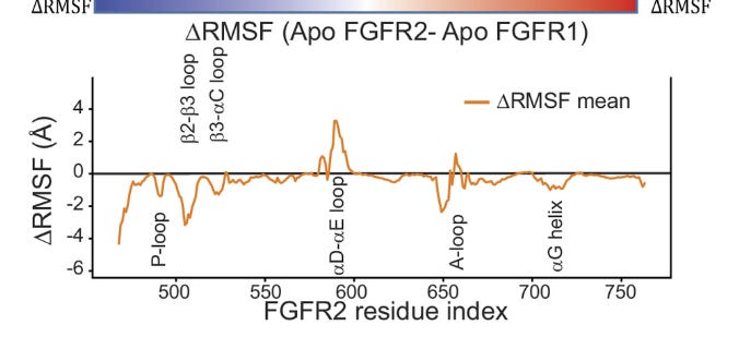
There’s something quite special here, MD revealed something — a conformational difference — that would’ve required much more expensive methods (like cryo-EM) to find! The authors continued down this rabbit-hole, hypothesizing how targeting the P-loop affected FGFR1 and FGFR2:
Our initial design efforts aimed to covalently engage FGFR2 Cys491, a residue that lies at the tip of the extended P-loop and is also targeted by the covalent pan-FGFRi futibatinib (10, 20, 21). Simulations of FGFR1 binding one of our early selective compounds suggested that its selectivity arose because the compound stabilized the FGFR1 P-loop in an extended conformation with such a low degree of flexibility that covalent engagement of Cys488 (homologous to FGFR2 Cys491) was discouraged.
In other words, targeting the P-loop may be a way to inhibit FGFR2 (bind to) but not FGFR1!
The paper goes on to use MD for docking purposes between potential molecules and binding to the P-loops of FGFR1 and FGFR2. This is a cool idea! But it’s also a bit hard to tell how useful MD was here, eyeballing the results don’t show huge differences in how ligands interacted with the P-loop, and they don’t attempt to calculate free energies anywhere. It feels likely that the key contributions of MD here were in identifying the P-loop as a selectivity handle and in providing post-hoc rationalization of the binding modes, rather than in directly guiding the docking itself.
Still though, a drug was made!
Using this approach as part of an iterative process of optimization, our efforts culminated in the identification of lirafugratinib (RLY-4008), a highly selective, orally available small-molecule FGFR2 inhibitor to enter clinical development.
Characterizing Receptor Flexibility to Predict Mutations That Lead to Human Adaptation of Influenza Hemagglutinin
Much more of an exploratory paper than an absolutely clinically useful one, but a great demonstration of the diversity of questions that MD can help answer.
Here’s the context: influenza pandemics occur when an (typically) avian influenza strain acquires mutations that allow it to infect and transmit between humans. A key step in this process is when the viral surface protein Hemagglutinin (or HA) switches its binding preference from avian to human sialic acid (SA) receptors via a mutation. However, predicting which specific mutations will enable this switch is challenging! One reason for this difficulty is that human SA receptors are quite flexible and can adopt many different conformations when bound to HA. This diversity makes it hard to determine from crystal structures alone which HA mutations will facilitate human receptor binding. An excellent use case for MD!
The simulations focused on a combination of SA’s and HA’s.
For SA’s (the cell surface receptor), 3-SLN, representing the avian sialic acid receptor, 6-SLN and 506-SLN, representing the human sialic acid receptors.
For HA’s (the viral protein), DK76, IN05, and SH13 were used. Along these, there were also several mutated forms of these HA’s used:DK76Q226L,G228S,A227S , DK76Q226L,G228S,P186N, DK76Q226L,G228S,P186N,A227S, DK76Q226L,G228S, DK76E190D,G225D IN05Q226L,G228S,S227A, IN05Q226L,G228S. Should these mutations mean anything to you? Some of these are just mutations that are known to ‘switch’ affinity of the viral protein between the human SA and the avian SA, and others are hypothetical gain-of-function mutations.
These were placed in cubic water boxes with periodic boundary conditions. The proteins were modeled using the Amber99SB-ILDN force field, while the GLYCAM06 force field was used for the sialic acid sugars — an example of multiple specialized force fields working alongside one-another. For each HA and SA combination, they ran simulations for up to 25 μs. The resulting set of trajectories (as in, every frame) were clustered together, yielding 7 clusters of identifiable conformations amongst all SA-HA pair frames (alongside an 8th ‘other’ category).
The rest of the analysis of this is…confusing. Probably not to someone who studies MD! But given what we’ve learned so far, hard to grasp. They come up with a way to measure binding affinity without relying on free energy differences — likely assisted by how long-running the simulation is, as they are able to directly observe many binding-unbinding events — and assert that their MD-derived numbers match up quite well with experimentally determined binding affinity values. They confirm this by suggesting a mutation to an HA to increase affinity and seeing that both MD and experimental validation both show an increase in binding affinity.
But I took the liberty of plotting their Kd values (binding affinity) derived from MD (KD_MD) and experimentally-determined (KD_MST) across multiple HA-SA pairs and…I’m not really seeing a strong correlation? There are a few cases in which it clearly works, but overall it feels quite random, outside of one outlier case. I’ve added a Github gist here of the (very basic) plotting work. It feels like the one-off de-novo mutation showing increased binding affinity in both MD and experimental techniques was either spurious or something that is real, but only works in some situations. I could very much be wrong about this though, please let me know if there’s something I’m missing!

Overall, very interesting hypothesis and cool how large conformational diversity was observed in both experimental determined structures AND in MD! But the binding affinity part of the paper was a bit off, unsure on whether I’m misunderstanding something or the results in this particular area are quite weak.
Conclusion
We covered the key components of an MD workflow - defining the system, choosing a force field, energy minimization, running the production simulations. We also looked at a few miscellaneous items, like quantum effects, enhanced sampling, and free energy calculations. Finally, we looked at a few papers, and saw cases of the jargon we’ve been learning this whole time being used to build useful atomic simulations.
But seven-thousand words later, I've only scratched the surface here! There are endless rabbit holes to dive down - coarse-grained simulations, more information on enhanced sampling, modifying the pH in simulations, and so on. But hopefully this post has given you a solid foundation to build on.
MD isn’t perfect and will likely remain imperfect for years to come. The timescales are still severely limited compared to biological reality. Quantum effects are largely ignored, even using approximate QM methods is hard. Force fields are approximations and there's no clear "best" choice. Setting up and running simulations requires a ton of expert knowledge.
But the future is interesting!
Things like neural force fields, trajectory sampling using Alphafold2-esque models, and trajectory interpolation using neural nets are all on the horizon and could lead to a revolution in the way we work with MD. Hopefully I get a chance to write about some of these directions someday! For now, it’s early days with these methods, and nothing has popped out as immediately, groundbreakingly useful. But, as with everything in biology-ML, things could shift overnight.
"Because MD time-steps are limited to femtoseconds — due to increasing instability and inaccuracy upon integrating Newton’s second law if pushed beyond that..."
There are some interesting things that go into the fs timescale stability limit, and even getting stable 2fs timesteps is nontrivial. In particular, when you discretize the time of your simulation you come up against the Nyquist–Shannon sampling theorem — essentially if you want to approximate the continuous time dynamics of your system, then you need to take small enough timesteps to capture the fastest timescales of motion. If you just naively set up your system, then you run into a real problem with hydrogen.
Because hydrogen is so light, H-X bond-length vibrations have a period of ~10fs. If you were to take ~10fs timesteps, then you could very easily ‘clip’ a hydrogen into its bonded partner, leading to VdW forces blowing the atoms apart on the next simulation step. Instead, you need to take ~0.1 fs or so timesteps so that you correctly model these vibrations — rough. A simple way to fix the above problem is just to treat the H-X bond length as fixed (e.g. the SHAKE / RATTLE algorithms), then you have no bond-length vibrations, and now you can worry about the next fastest timescale in your system (hint, still hydrogen)! This is the default setting in most MD software, and usually allows for stable ~2fs timesteps for biomolecule simulations in water.
Even having fixed the H-X bond lengths, the torsional period of hydrogen e.g. H-C-H is ~100fs, contributing to instability when you integrate over timesteps larger than 2fs. We can’t apply the same fix as last time, since simply fixing these torsion angles would make simulated molecules behave super unrealistically. A clever trick people use is to instead do something called ‘hydrogen mass repartitioning’ (HMR), in which you distribute some of the mass of the heavy partner in the H-X bond into the hydrogen atom — e.g. often the hydrogen mass is set to 2 amu, in which case each hydrogen in an H-X bond ‘borrows’ 1 amu of mass from its heavy partner. This more-or-less maintains the centre of mass / moment of inertia etc of most molecules, but effectively doubles the natural period of fast motions like H-X-H bond torsions, often allowing for a doubling of the stable timestep to 4fs. This seems kinda lame, but when your simulations take on the order of days we take these wins. This does make hydrogens behave differently in simulation, and so depending on what kind of systems / interactions the MD simulations are being used to study this isn’t always a great option, so 2fs is more or less the granularity of 95% of MD work on proteins.
"And that’s it! We now know the updated velocity and position at the next time step, we just need to do this a few **million** times and our simulation is complete! Over very many hours of compute time, we’ll end up a massive stack of data known as a trajectory, which will encode the position and velocities for every particle in our system from timestep-to-timestep, showing the molecular dance that occurs. The video below is an accurate representation of how our folded protein's trajectory may look (start at 0:15). Lots of vibrating around, slowly poking its way towards a stable structure, and then fully stabilizing — all over 6 **million** femtoseconds (6 microseconds)."
Both times that should be **billion** rather than million. 6 million femtoseconds are 6 nanoseconds. 6 billion femtoseconds are 6 microseconds.